Writing a search engine is hard. When confronted with the endless complexities of language, it is usually best to use code written by other, presumably smarter, people. For whatever reason, I was recently forced to implement my own search engine. Although this might have been accomplished with sufficient guesswork, I decided to try and derive an appropriate algorithm with math! I’ve documented my approach here if anyone else ever finds themselves in a similar situation.

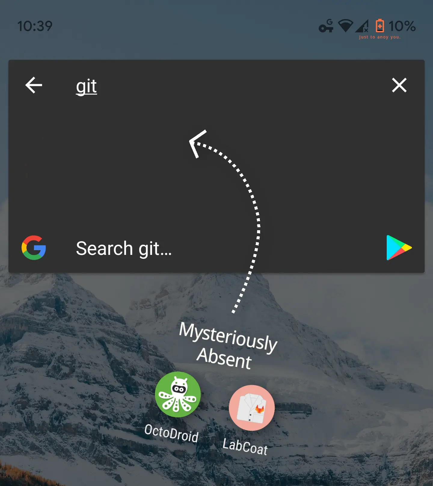
Before we begin, we need some data to search. I am endlessly annoyed that searching “git” on my phone doesn’t bring up either the “OctoDroid” or “LabCoat” apps, so let’s reinvent my app drawer.

Constructing a Model

I use my app drawer’s search bar when I want to find and open a specific app that is otherwise buried in a sea of little circle icons. So the drawer should really be trying to guess what app I want to open. Apps that are more likely should come first and apps that are not at all likely should be left out entirely.

Before I type a single letter, our search algorithm can already make some reasonable guesses. Most of the time I am just going to select Firefox, Google Maps, or Reddit. Those apps should start out at the top of the drawer. Only once I type “g” should git-related apps start moving up.

Conditional Probability

The probability that I select an app A , before typing anything, is called the “prior probability” and written P(A) . Once we have some more evidence of my intentions (in the form of me typing some search query Q ), we want to use use the probability of “ A given that evidence” which is written as P(A \mid Q) . This is called conditional probability. So, how do we calculate conditional probability? In this case, we will use a little recipe called Bayes’ Rule, which says that:

\begin{aligned} P(A \mid Q) = \frac{P(Q \mid A) \; P(A)}{P(Q)} \end{aligned}

We already know how to estimate P(A) (the prior probability that I am looking for A no matter the query). Simply track how often I open each app.

But what is P(Q) ? That’s the probability of me typing some query Q no matter the app I’m looking for and it is a little tricky to estimate. Thankfully, we can come back to it later since it isn’t needed to simply rank apps relative to each other. P(Q) depends on the query only and so effects the probability of A \mid Q for each app A equally.

So all we need now is P(Q \mid A) ! What is P(Q \mid A) ? Well, if P(A \mid Q) is the probability of me looking for A given I have typed Q , then P(Q \mid A) must be the probability of me typing Q given I am looking for A . To calculate this probability, let’s think through a hypothetical sequence of events:

I am looking for “LabCoat”
Since “LabCoat” is an app for managing git repositories, I think “git”
I start by typing the letters “gi”

There are now a bunch more probabilities we need to deal with:

\begin{aligned} P(A) &= \text{How likely is it that am looking for LabCoat?} \\[1em] P(K \mid A) &= \text{How likely is it that I will think ``git'' when looking for LabCoat?} \\[1em] P(Q \mid K) &= \text{How likely is it that I will type ``gi'' when thinking ``git''?} \\[1em] \end{aligned}

Conceptually, typing “gi” is evidence that I am thinking “git” which in turn is evidence that I am looking for LabCoat. By applying some rules of conditional probability to Bayes’ Rule above (which is left as an exercise for sufficiently bored readers), we get:

\begin{aligned} P(A \mid Q) = \frac{\sum_K P(Q \mid K) \; P(K \mid A) \; P(A)}{P(Q)} \end{aligned}

In human-speak, this equation says:

“The likelihood that I am looking for some app is proportional to the similarity of the query to a keyword times the relevance of that keyword to the app summed over all relevant keywords.”

The term P(K \mid A) is fairly easy. It is just a metric for how relevant K is as a keyword for A . If LabCoat has n keywords of equal weight, then P(K \mid A) = \frac{1}{n} . If some keyword is stronger, then we can give it a little more probability and the others a little less.

But it is still a unclear how we should estimate P(Q \mid K) . I did this by borrowing the concept of an “edit” which is some alteration from one item of text to another.

Edit Distance

Let’s suppose I think the word “firefox” but then type “frefo”. To a human it is pretty easy to guess what happened, but how can a computer guess? If you remember your college computer science courses you may be screaming “use the the Levenshtein distance!” at your screen. However, the goal of this blog post is to derive a search algorithm from first principals. So if we want to use the the Levenshtein distance (or a similar edit-distance metric), we will have to justify it mathematically.

Let’s define E as a sequence of edits which is made of individual alterations E_1, E_2, \dots, E_n . The probability P(E) is simply the likelihood of all E_1, E_2, \dots, E_n occurring. Some alteration E_i might be very likely if it is just me leaving some letters off the end of a word (afte al, typin is so borin) but less likely if it is something like replacing “i” with “q”.

But how does P(E) relate to P(Q \mid K) ? Let’s define P(Q \mid K, E) which is the probability of me typing Q when I meant to type K but made edits E . If E does indeed change K into Q , then the probability is 100%. When those edits are applied to that keyword it will always result in the query. Otherwise the probability is 0.

Now from the rules of probability, we can get:

P(Q \mid K) = \sum_E P(Q \mid K, E) \; P(E)

See how the term P(Q \mid K, E) just acts like a filter, so that we sum only the probabilities of all edits that change K into Q ? For example, to calculate the probability that we type “firefox” as “frefo”, we sum the probabilities of:

Deleting the “i” and the “x”.
Deleting “ox” and replacing “iref” with “refo”.
Inserting an “f”, deleting “fo”, and deleting “x”.
…

But conceptually this equation calculates a sum, not the minimum, which prevents us from using the traditional algorithm for edit distance. And these aren’t really distances (1 edit, 2 edits, etc) at all but probabilities (1%, 30%, etc). What is going on?

Negative Log

Let’s take a break from math and think about how we might implement this algorithm so far (an exercise I may attempt in a later post). Throughout this process we keep multiplying small probabilities together to get even smaller probabilities. Like, what is the chance of replacing “iref” with “refo”, out of all the mistakes I could possibly make? Even randomly forgetting an “i” is pretty unlikely. And with all the apps on my phone, how often do I open an app to, say, change my wallpaper? We are running into dangerous floating-point-precision territory here. The probabilities of making specific queries could be on the order of 10^{-8} or less for anything but a perfect match.

Maybe we should be using exponential notation? We could take the negative log of each probability. So instead of saying P(E) = 0.000000001 we will say -\log(P(E)) = I(E) = 8 . Because of the precision benefits, using log probability is a pretty common practice in computer science. The notation of I instead of P as comes from information theory, where the log probability is called “information content” or “surprise”. Information theorists would also tell us that if we use base 2, our log probabilities will be in units of bits! But what does all that do to our math?

\begin{aligned} I(E) &= I(E_1 \wedge E_2 \wedge \dots \wedge E_n) \\[1em] &= -\log[P(E_1) \times P(E_2) \times \dots \times P(E_n)] \\[1em] &= I(E_1) + I(E_2) + \dots + I(E_n) \\[1em] &= \text{sum of penalties for each individual alteration} \\[1em] &= \text{the ``distance'' of } E \end{aligned}

Cool! Products become sums and we are one step closer to using the edit distance. And what happens to sums like P(Q \mid K) = \sum_E P(Q \mid K, E) P(E) ? Unfortunately there is no simple way to do the log of a summation. But what are the terms in that summation? The probabilities of different, increasingly convoluted edits. As the edits get more convoluted they require exponentially more unlikely alterations. So most of the edits in that sum are massively less probable than the most probable edit and contribute little to the total. In fact, the log of a sum is used in machine learning as a soft approximation of maximum. Thus, the log of this sum is well approximated by the log probability of the maximally probable edit (the one with the lowest log probability):

I(Q \mid K) \approx \min_E \; I(E) \approx \min_E \; I(E_1) + I(E_2) + \dots + I(E_n)

Voilà, I(Q \mid K) is well approximated by the minimum edit distance between Q and K ! This approximation works well for other sums in our algorithm. So long as we assume each query is much closer to one keyword than to the others, we now have:

\begin{aligned} I(A \mid Q) \approx \min_{K, E} \; I(E_1) + I(E_2) + \dots + I(E_n) + I(K \mid A) + I(A) - I(Q) \end{aligned}

And as discussed above, we can leave out the P(Q) term if all we need is a relative score. At last, we have a mathematically derived scoring function for our search algorithm:

\texttt{score} (A, Q) = \min_K \; \texttt{edit\_distance} (K, Q) + I(K \mid A) + I(A)